Prereqs and notational matters
This post requires a basic understanding of the potential outcomes framework and familiarity with the standard notation; see our earlier post for the necessary background and notation.
Appropriate notation is critical in causal inference, as it can give a visual reminder of some of the subtlety involved. The key challenge is to strike an appropriate balance between mathematical rigor, which would make the notation precise but heavy and sometimes hard to parse, and simplicity, which would make it readable at the cost of the occasional ambiguity. Another complication is that some unfortunate notational habits have become de facto standard in the literature, making their use almost unavoidable. We do our best to use clear and sensible notation while hewing close to the generally accepted standard.
In our first post on the subject, we used a number of notational crutches that were appropriate for an introduction to the subject, but will quickly become cumbersome. For instance, we denoted vectors with the arrow symbol (e.g., \(\vec{W}\) and \(\vec{Y}\)): these are now omitted. We also drop the superscript ‘‘DiM’’ from the difference-in-means estimator \(\hat{\tau}\) and the superscript ‘‘ATE’’ from the average treatment effect estimand \(\tau\).
The question of inference
How good is my guess?
Consider a randomized experiment run on a population of \(n\) units to assess the effect of a binary intervention; assume throughout that there is no interference.
To make things very concrete, suppose that \(n=6\) and that we observe the assignment \(W = (1, 1, 0, 1, 0, 0)\) and the outcome vector \(Y = (3, 1, 2, 1, 3, 0)\). Suppose our goal is to estimate the Average Treatment Effect (ATE),
\[ \tau = \frac{1}{6} \sum_{i=1}^6 \bigg(y_i(1) - y_i(0)\bigg), \]
using the observed data. One possible solution is to use the difference-in-means estimator,
\[ \hat{\tau} = \frac{1}{3}( 3, 1, 1) - \frac{1}{3}(2, 3, 0), \]
which gives us an estimate of \(\hat{\tau} = 0\) for \(\tau\). As we’ve seen in our introduction to the potential outcomes framework, an estimator is a data-driven ‘‘guess’’ of the value of an estimand. The difference-in-means estimator is one procedure for obtaining such a guess and, presently, it gives us a guess of \(0\) for the ATE.
But, how good a guess is this? We could have guessed 42, -5, or 1380. Why should \(0\) be preferred, given the data we observed? The answer to this question is complex, and it is at the heart of what statistical inference is.
A parametric answer
If you have taken an introduction to statistical inference, then your answer might start with the assumption that:
\[
\begin{aligned}
Y_i \mid W_i = 1 \,\, &\overset{iid}{\sim} \,\, N(\mu_1, \sigma_1^2) \\\
Y_i \mid W_i = 0 \,\, &\overset{iid}{\sim} \,\, N(\mu_0, \sigma_0^2) \\\
\end{aligned}
\]
It is easy to show that the difference-in-means estimator \(\hat{\tau}\) is the Maximum Likelihood Estimator (MLE) for the parameter \(\theta \equiv \mu_1 - \mu_0\). But that is an awkward answer for a number of reasons:
- Since by definition, \(Y_i = W_i \, y_i(1) + (1-W_i) \, y_i(0)\), assuming that \(Y_i \mid W_i = 1\) and \(Y_i \mid W_i = 0\) follow some distributions implies that \(y_i(1)\) and \(y_i(0)\) must be random. This in turns implies that the science table \(\underline{y} = (y(1), y(0))\) is random, and therefore our estimand \(\tau\) is itself a random variable! So it’s all nice and good to say that \(\hat{\tau}\) is the MLE for the parameter \(\theta\), but what does the parameter \(\theta\) have to do with the random variable \(\tau\)?
- The parameter \(\theta \) is also a population parameter; that is, to interpret it, we implicitly require the assumption that there exists some larger population from which we sample our experimental units. This sampling allows us to model the outcomes as random; however, the price we pay is that our inference makes claims about the larger population, NOT our actual sample!
- Our key building blocks, in the potential frameworks, are… well, the potential outcomes — not the observed outcomes! The distributions on \(Y_i \mid W_i = 1\) and \(Y_i \mid W_i = 0\) imply assumptions on the distributions \(y(1)\) and \(y(0)\), but these are not transparent.
Both points can be partially addressed by modifying the assumption as follows:
\[
\begin{aligned}
Y_i(1) \, \, &\overset{iid}{\sim} N(\mu_1, \sigma_1^2), \\\
Y_i(0) \, \, &\overset{iid}{\sim} N(\mu_0, \sigma_0^2), \\\
W_i \,\, &\perp \,\, (Y_i(1), Y_i(0)),
\end{aligned}
\]
where \( \perp \) is used to indicate that \(W_i\) and \((Y_i(1), Y_i(0))\) are independent.
Under these specifications, \(\hat{\tau}\) is still
the MLE for \(\theta = \mu_1 - \mu_0\), but now we can also establish a
connection between \(\theta\) and \(\tau\):
\[ E[\tau] = \theta, \] where the expectation is taken with respect to the distribution of the potential outcomes.
With some work, we can state analogous results without assuming normality, but we still require that the potential outcomes be independent and identically distributed. This may seem like a mild assumption, but it is still an assumption — and in some scenarios (e.g.,in the presence of interference), it is anything but mild. In addition, we started with \(\tau\) as our estimand, but we had to settle for \(\theta\) which, even if it is connected to \(\tau\), is not what we were originally after.
It turns out that we don’t need to assume anything about the potential outcomes to say something meaningful about \(\tau\). Unlike traditional statistical inference problems, experiments have an additional source of variability: the random assignment. To use this for inference requires thinking about the problem in a somewhat unique way, as we see below.
Randomization as the basis for inference
Our goal is to limit the number of necessary assumptions so that our conclusions can be as objective as possible. To begin with, let’s focus on the one element that we control: the assignment mechanism. Let’s say that the assignment mechanism is a completely randomized design with parameter \(n_1 = 3\), as defined in our previous post. Then, all the assignments with exactly \(3\) treated units and, therefore, \(3\) control units have equal probability, while all other assignments have probability \(0\).
Let’s see how far we can go with just this simple assumption. As before, we consider the science table to be a constant \(\underline{y} = (y(0), y(1))\). For illustration purposes, let’s take \(\underline{y}\) to be as follows:
| i | \(y_i(0)\) | \(y_i(1)\) |
|---|---|---|
| 1 | 2 | 3 |
| 2 | 1 | 1 |
| 3 | 2 | 4 |
| 4 | 0 | 1 |
| 5 | 3 | 3 |
| 6 | 0 | 2 |
In practice, the science is unknown (if we knew it, why would we be running an experiment?) — here, we give it a concrete value just to illustrate our point.
Now, say we observe the assignment \(W^{(1)} = (1, 1, 1, 0, 0, 0)\). Recall that we defined the observed outcome of unit \(i\) to be \(Y_i = W_i \, y_i(1) + (1-W_i) \, y_i(0)\), so the vector of observed outcomes becomes \(Y = (3, 1, 4, 0, 3, 0)\), and the difference-in-means estimator is:
\[ \hat{\tau}^{(1)} = \hat{\tau}(W^{(1)}) = \frac{1}{3} (3 + 1 + 4) - \frac{1}{3} (0 + 3 + 0) = \frac{5}{3}. \]
Note: Mathematically, the estimator \(\hat{\tau}\) is a function of both the assignment \(W\) and the outcome vector \(Y\). Since \(Y\) is itself a function of \(W\) and the science \(\underline{y}\), we could write \(\hat{\tau} = \hat{\tau}(W, \underline{y})\), with the understanding that it is a function that can be computed from observed data since the dependence on \(\underline{y}\) is only through the observed \(Y\). Ultimately though, since we consider the science table \(\underline{y}\) as fixed and unknown, we keep it implicit in our notation for the estimator and simply write \(\hat{\tau}(W)\).
What happens if we had observed a different assignment? For instance, say we observed the assignment \(W^{(2)} = (1, 0, 1, 0, 1, 0)\), then we would have observed the outcome vector \(Y = (3, 1, 4, 0, 3, 0)\), and the difference-in-means estimator would have had the value:
\[ \hat{\tau}^{(2)} = \hat{\tau}(W^{(2)}) = \frac{1}{3} (3 + 4 + 3) - \frac{1}{3} (1+0+0) = 3. \]
Now since we consider a completely randomized design with parameter \(n_1 = 3\), both assignments \(W^{(1)}\) and \(W^{(2)}\) have equal probability of being observed
\[ pr(W^{(1)}) = pr(W^{(2)}) = \frac{1}{6 \choose 3}. \]
The random variable \(\hat{\tau}\), therefore, takes the value \(\frac{5}{3}\) with probability \({6 \choose 3}^{-1}\) and the value \(3\) with probability \({6 \choose 3}^{-1}\). If we repeat this with all \(6 \choose 3\) possible values of the assignment vector, we obtain the distribution of \(\hat{\tau}\) induced by the assignment mechanism \(pr(W)\). Formally, for \(t \in \mathbb{R}\), we define
\[ pr(\hat{\tau} = t) \equiv \sum_{w} \mathbb{I}[\hat{\tau}(w)=t]\,\, pr(W = w) \]
where the function \(\mathbb{I}[\cdot]\) is an indicator that takes value \(1\) if whatever is inside it is true, and value \(0\) otherwise.
In summary, if we knew the entire science table \(\underline{y}\), we could build the following table, which summarizes the distribution \(pr(\hat{\tau})\).
| k | \(W^{(k)}\) | \(\hat{\tau}(W^{(k)})\) |
|---|---|---|
| 1 | \((1,1,1,0,0,0)\) | \(\frac{5}{3}\) |
| 2 | \((1,0,1,0,1,0)\) | \(3\) |
| … | … | … |
| \(6 \choose 3\) | \((0,0,0,1,1,1)\) | \(\frac{1}{3}\) |
If you think about it, this table provides a lot of information! For example, it lets us compute our estimator’s expectation and variance—two rather valuable quantities. Of course, we don’t know the entire science table. Therefore we never see the previous table — or to be more specific, we only ever observe a single row from that table: this is yet another manifestation of the fundamental problem of causal inference.
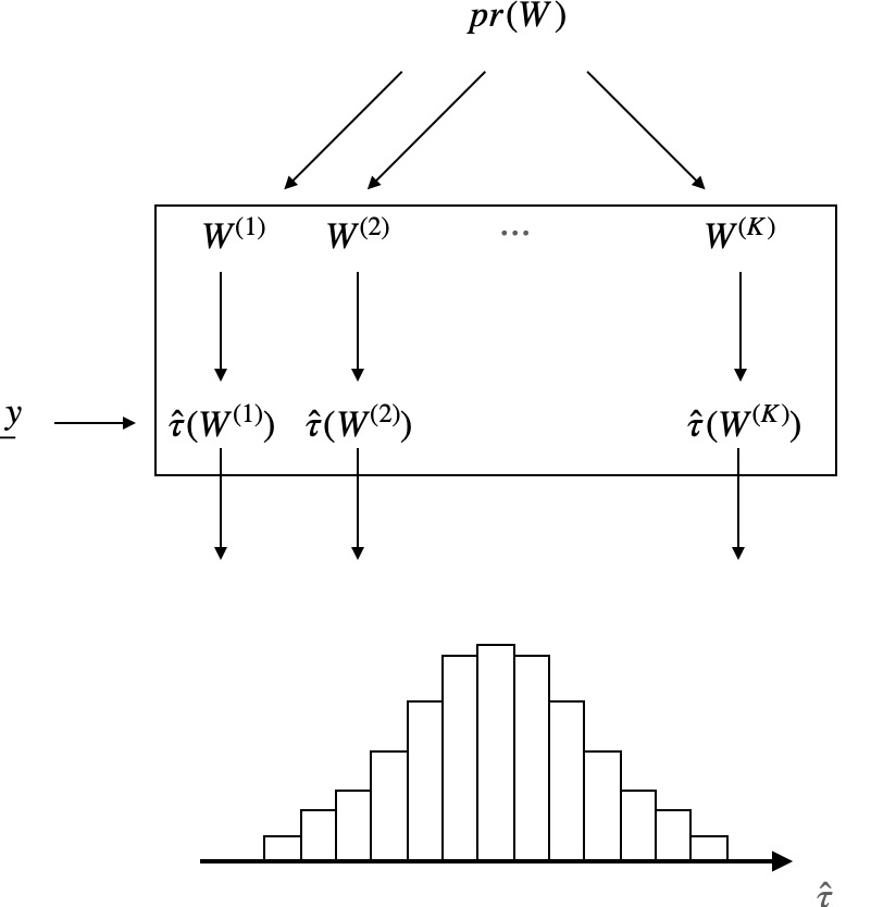
The figure illustrates pr(W) as the source of randomness and provides another visual of the above table.
Neymanian inference
The general inferential strategy we discuss in this post is named after the famous statistician Jerzy Neyman. It leverages the ideas directly from the previous section by focusing on the properties of the estimator. Indeed, we have seen that \(\hat{\tau}\) is a random variable whose distribution is induced by the assignment distribution \(W \sim pr(W)\). It therefore makes sense to consider quantities like the expectation \(E[\hat{\tau}]\) of \(\hat{\tau}\) as well as the bias of \(\hat{\tau}\) for estimating \(\tau\).
Let’s start with the expectation, because it is helpful in reinforcing how randomization inference works. For an assignment mechanism \(pr(W)\), define \(\mathbb{W} = \{W: pr(W) > 0\}\) the support of the design, and denote by \(\mathbb{T} = \{\hat{\tau}(w), w \in \mathbb{W}\}\) the set of all distinct values the estimator can take. By definition we have,
\[ E[\hat{\tau}] = \sum_{t \in \mathbb{T}} t \, \cdot \, pr(\hat{\tau} = t), \]
The following equivalent formulation is often more convenient
\[ E[\hat{\tau}] = \sum_{t \in \mathbb{T}} t \, \cdot \, pr(\hat{\tau} = t) = \sum_{w \in \mathbb{W}} \hat{\tau}(w) \, \cdot \, pr(W = w). \]
As we discussed, since we don’t know the science table, we only observe a single realization from the random variable \(\hat{\tau}\), corresponding to a single draw from the distribution \(pr(\hat{\tau})\). It turns out, however, that we can say a lot about \(pr(\hat{\tau})\) even if we only observe the estimate \(\hat{\tau}(W)\) corresponding to the observed assignment \(W\), as long as we know the assignment mechanism \(pr(W)\).
For instance, in the previous post, we stated the following proposition:
Proposition: If \(W\) is assigned according to a completely randomized design, then the difference in means estimator \(\hat{\tau}\) is unbiased for the average treatment effect \(\tau\).
Below we provide a formal proof of this result to give a sense of how the math works. Even if you’re not super interested in the maths, we strongly recommend that you take a close look, as it will help you understand randomization-based inference better.
Proof: The goal, stated in mathematical terms, is to show that:
\[ E[\hat{\tau}] = \tau. \]
We’ll do that in four steps.
(1) Recall from basic probability that the expectation is linear,
\[
\begin{aligned}
E[\hat{\tau}] &= E\bigg[\frac{1}{N_1} \sum_{i=1}^N W_i Y_i - \frac{1}{N_0}\sum_{i=1}^N (1-W_i) Y_i \bigg] \\\
&= \frac{1}{N_1} \sum_{i=1}^N E[W_i Y_i] - \frac{1}{N_0} \sum_{i=1}^N E[(1-W_i) Y_i].
\end{aligned}
\]
(2) Now the tricky part is that both \(W_i\) and \(Y_i\) are random variables, so we cannot write \(E[W_i Y_i] = E[W_i] E[Y_i]\) a priori. The key is to notice that since by definition \(Y_i = W_i y_i(1) + (1-W_i) y_i(0)\), we have:
\[ W_i Y_i = W_i^2 y_i(1) + W_i (1-W_i) y_i(0) = W_i y_i(1). \]
This helps because \(y_i(1)\) is a constant, so
\[ E[W_i Y_i] = E[W_i y_i(1)] = E[W_i] y_i(1). \]
(3) Finally, recall from basic probability that if \(W_i\) is a binary random variable, \[ E[W_i] = P(W_i = 1) = \frac{N_1}{N} \] where the second equality follows from the fact that the design is completely randomized. So, all together, we have: \[ E[W_iY_i] = \frac{N_1}{N} y_i(1) \] An exactly parallel derivation shows that: \[ E[(1-W_i)Y_i] = \frac{N_0}{N} y_i(0) \]
(4) Putting it all together, we have:
\[
\begin{aligned}
E[\hat{\tau}] &= \frac{1}{N_1} \sum_{i=1}^N \frac{N_1}{N} y_i(1) - \frac{1}{N_0} \sum_{i=1}^N \frac{N_0}{N} y_i(0) \\\
&= \frac{1}{N} \sum_{i=1}^N y_i(1) - \frac{1}{N} \sum_{i=1}^N y_i(0) \\\
&= \tau
\end{aligned}
\]
which completes the proof.
If you think about it, this result is admirable. We have indeed made no assumption whatsoever on the potential outcomes \(\underline{y}\) — these could be anything. The only assumption made in this proposition is that the treatment was assigned in a particular random way. But since the assignment mechanism \(pr(W)\) is presumably under our control, this is not much of an assumption: the proposition tells us that if we run our experiment a certain way, the difference-in-means estimator \(\hat{\tau}\) will be unbiased.
Now unbiased estimators are good, but knowing that an estimator is unbiased gives us only a partial picture of its performance. What we really want is a measure of our uncertainty, as provided by confidence intervals (or credible intervals, for Bayesians). Incredibly, it turns out that we can construct such intervals with the difference-in-means estimator and prove that they are valid for the ATE while making only a few very mild assumptions. In particular, we still don’t need to assume that the potential outcomes are independent or identically distributed (or, indeed, even random). The pseudo-theorem below gives you a high-level picture of the kind of result that can be derived:
Pseudo-theorem: Suppose that \(pr(W)\) is a completely randomized design. Then we can construct an interval \(\widehat{CI} = \widehat{CI}(Y, W)\) that depends only on observed quantities, such that under mild conditions, \[ pr(\tau \in \widehat{CI}) \geq 0.95 \] for large \(n\). The interval \(\widehat{CI}\) is therefore a valid \(95\%\) confidence interval for the average treatment effect \(\tau\).
Although stated rather informally, this is a beautiful result. It essentially says that one can construct valid confidence intervals for the ATE without assuming much about \(\underline{y}\) if one controls the assignment mechanism. Stating this result formally requires some more technical tools and concepts that are beyond the scope of this introductory post: we will tackle them in a subsequent article in this series.
Convince yourself!
The ideas presented in this post are not difficult, but they may feel unfamiliar to many — because they are! We have seen two main sources of confusion in students seeing this material for the first time:
- Understanding what is random and what is not.
- Understanding what is observed and what is not.
The best way to become comfortable with randomization-based inference — and convince yourself that there is no magic involved — is to play around with small simulations.
The R code below illustrates the example we considered throughout this post. You
can also find on github. Go ahead and modify the values of the potential outcomes in the
science table on lines 23 and 24 (making sure to keep them of length 6, so the rest
of the code works unchanged). You will see that if you modify the science, the
value of the variable tau will change, but the value of bias will
remain equal to 0, up to numerical precision!
| |