What is causal inference?
Causal inference is a vast field that seeks to address questions relating causes to effects. We more formally (but still not very rigorously) define causal inference as the study of how a treatment (aka action or intervention) affects outcomes of interest relative to an alternate treatment. Often, one of the treatments represents a baseline or status quo: it is then called a control. Academics have used causal reasoning for over a century to establish many scientific findings we now consider as facts. In the past decade, there has been a rapid increase in the adoption of causal thinking by firms, and it is now an integral part of data science.
Examples: causal questions
- What is the effect on the throughput time (outcome) of introducing a new drill to a production line (treatment) relative to the current process (control)?
- What is the effect of changing the text on the landing page’s button (treatment) on the clickthrough rate (outcome), relative to the current text (control)?
- Which of two hospital admission processess (treatment 1 vs treatment 2) leads to the better health results (outcome)?
The most reliable way to establish causal relationships is to run a randomized experiment. Different fields have different names for these, including A/B tests, clinical trials, randomized control trials, etc… but basically, a randomized experiment involves randomly assigning subjects (e.g., customers, divisions, companies) to either receive a treatment or a control intervention. The effectiveness of the treatment is then assessed by contrasting the outcomes of the treated subjects to the outcomes of the control subjects.
The simple idea of running experiments has had a profound impact on how managers make decisions, as it allows them to discern their customers’ preferences, evaluate their initiatives, and ultimately test their hypotheses. Experimentation is now an integral part of the product development process at most technology companies. It is increasingly being adopted by non-technology companies as well, as they recognize that experimentation allows managers to continuously challenge their working hypotheses and perform pivots that ultimately lead to better innovations.
Unfortunately, we cannot always run experiments because of ethical concerns, high costs, or an inability to control the random assignment directly. Luckily, this is a challenge that academics have grappled with for a long time, and they have developed many different strategies for identifying causal effects from non-experimental (i.e., observational) data. For example, we know that smoking causes cancer even though no one ever ran a randomized experiment to measure the effect of smoking. However, it is important to understand that causal claims from observational data are inherently less reliable than claims derived from experimental evidence and can be subject to severe biases.
This post provides a high-level overview of these two methods.
Observational Studies
The vast majority of statistics courses begin and end with the premise that correlation is not causation. But they rarely explain why we can not directly assume that correlation is not causation.
Does signing up to a premium account reduce music streaming?
Let’s consider a simple example. Imagine you are working as a data scientist for Musicfi, a firm that offers on-demand music streaming services. To keep things simple, let’s assume the firm has two account types: a free account and a premium account. Musicfi’s main measure of customer engagement is the total streaming minutes that measure how many minutes each customer spent on the service per day. As a data scientist, you want to understand your customers, so you decide to perform a simple analysis that compares the total streaming minutes across the two account types. To put this in causal terms:
- Our treatment is having a premium account.
- Our control is having a free account.
- Our outcome is total streaming minutes.
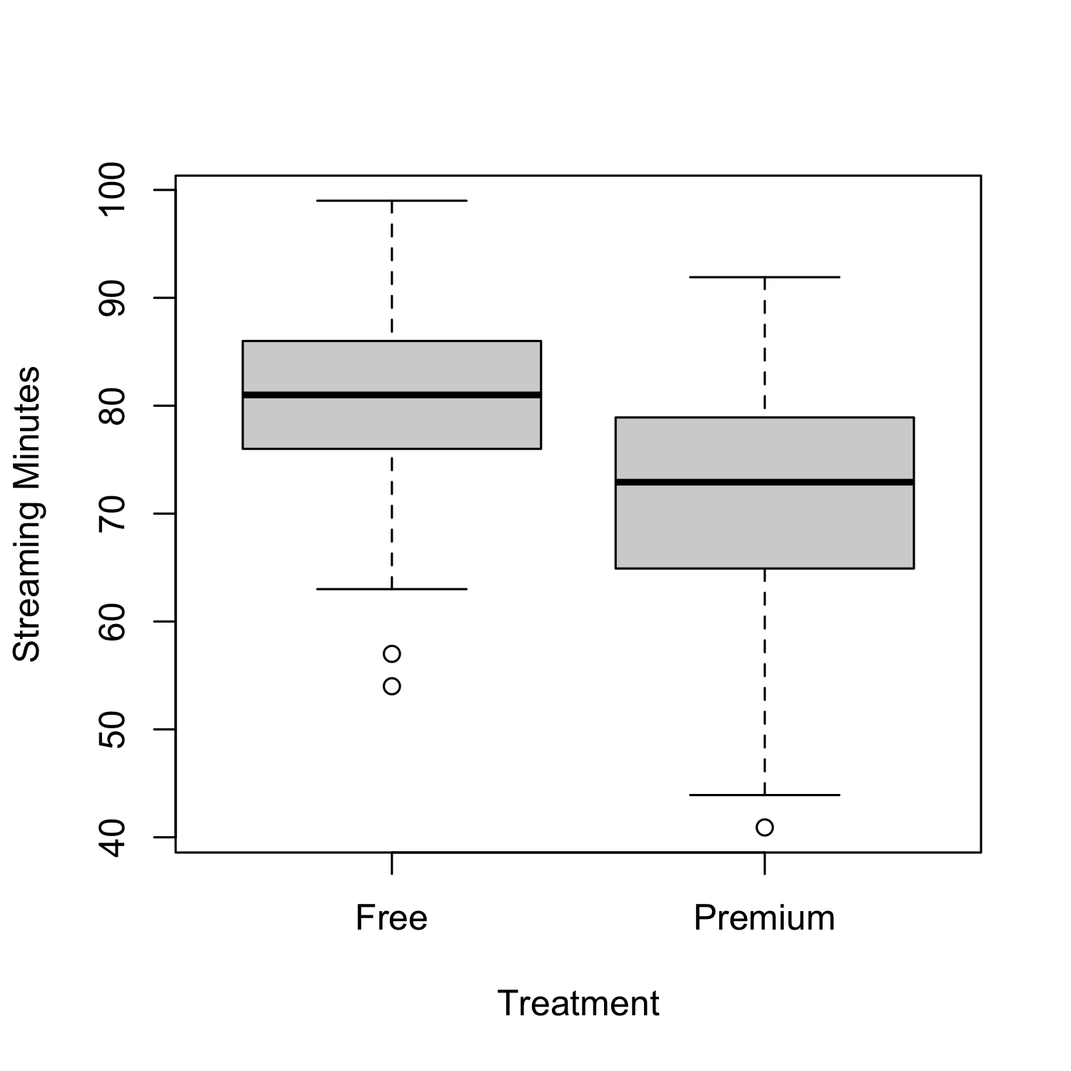
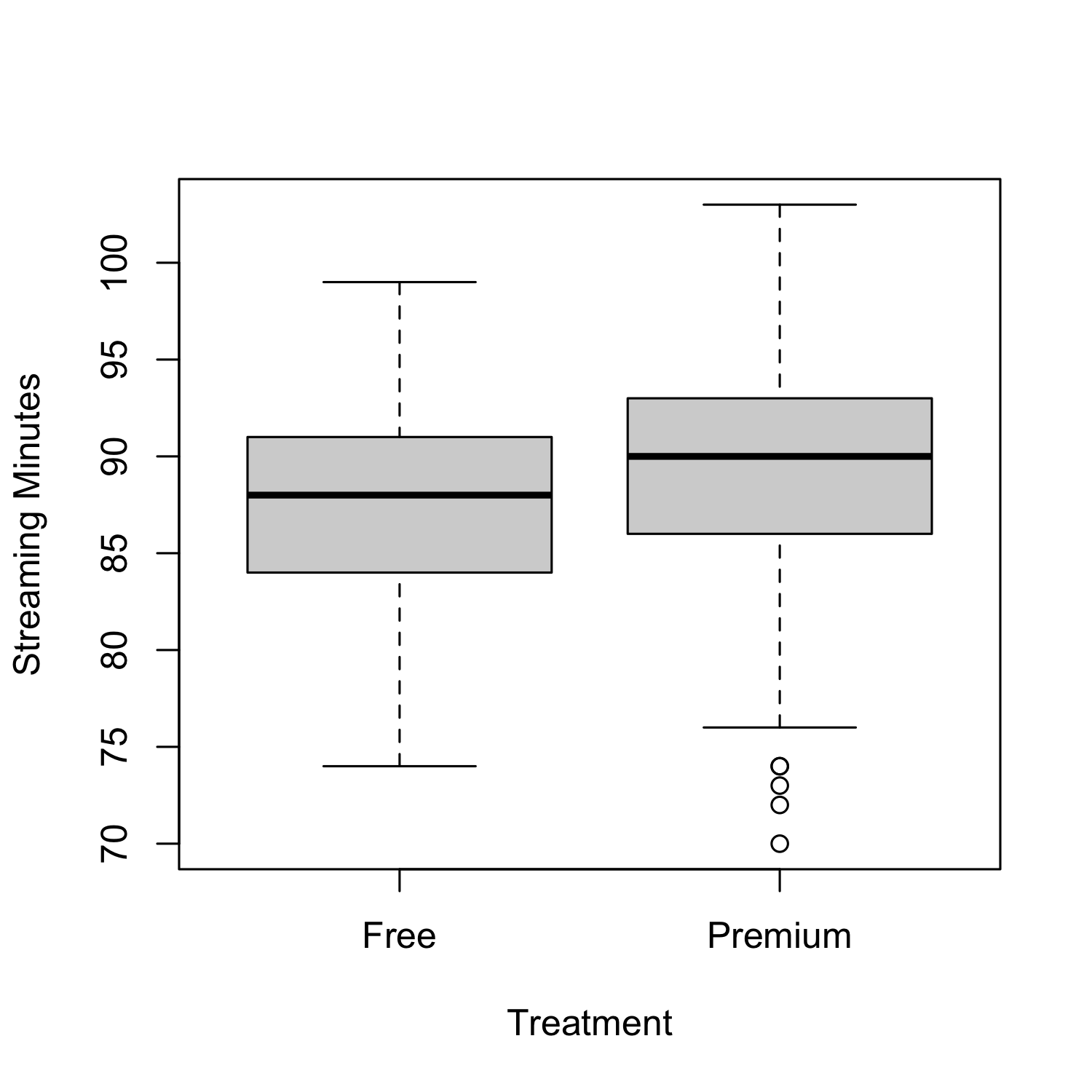
From the figure, we can see that the customers with premium accounts had lower total streaming minutes than customers with free accounts! The average in the premium group was 71 minutes compared to 81 minutes in the free group, meaning that (on average) customers with a premium account listened to less music!! We can use a t-test to check if this observed difference is statistically significant:
| |
Suppose we take the above results at face value. In that case, we might incorrectly conclude that having a premium account reduces customer engagement. But this seems unlikely! Our general understanding suggests that buying a premium account should have the opposite effect. So what’s going on? Well, we are likely falling victim to what is often called selection bias. Selection bias occurs when the treatment group is systematically different from the control group before the treatment has occurred, making it hard to disentangle differences due to the treatment from those due to the systematic difference between the two groups.
Mathematically, we can model selection bias as a third variable—often called a confounding variable—associated with both a unit’s propensity to receive the treatment and that unit’s outcome. In our Musicfi example, this variable could be the age of the customer: younger customers tend to listen to more music and are less likely to purchase a premium account. Therefore, the age variable is a confounding variable as it limits our ability to draw causal inferences.
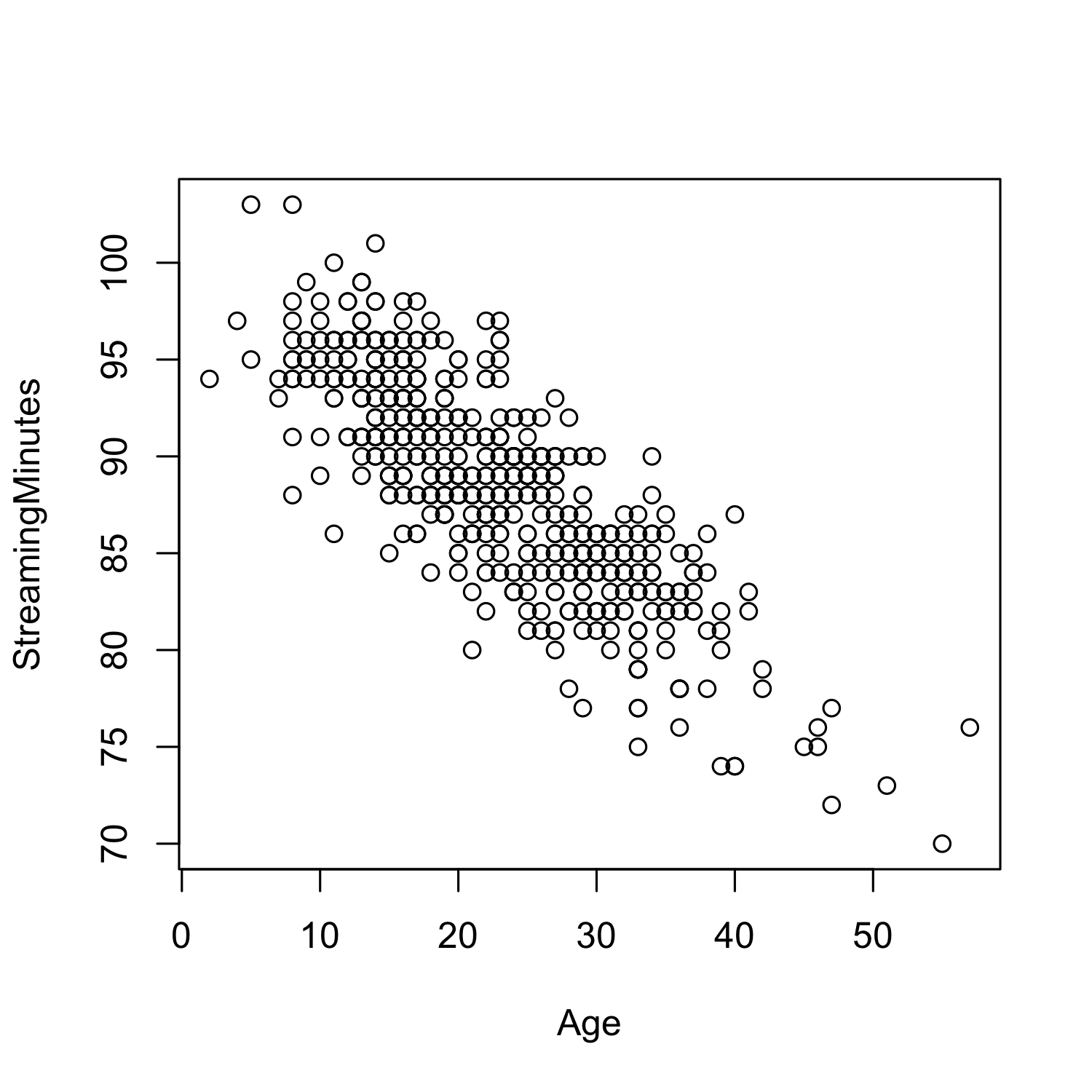
To see this, we can compare how age is related to total streaming minutes and the account type.
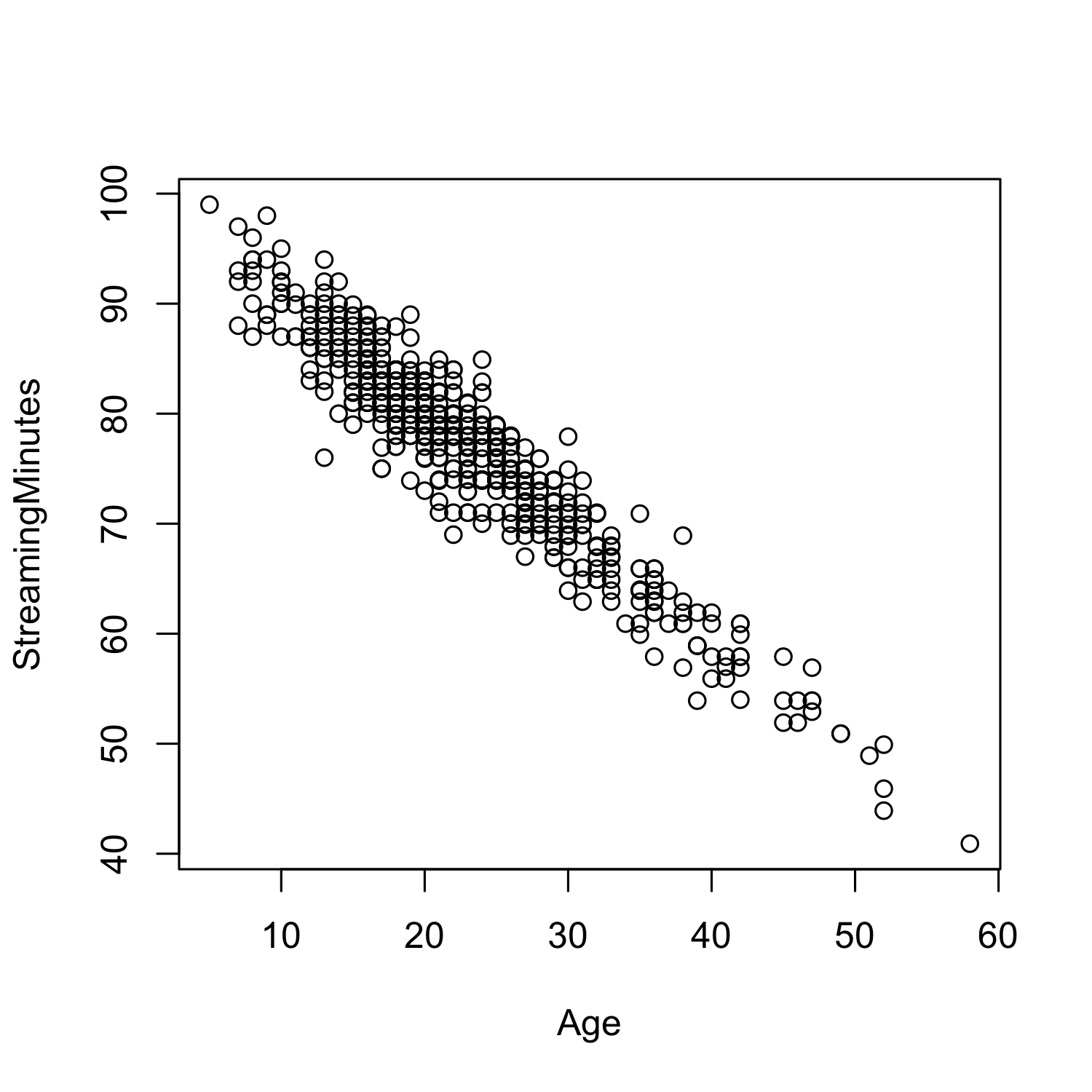
There is a clear relationship between Streaming Minutes and Age: Younger users stream a lot more than older users!
If we wanted to adjust for the age variable (assuming it is observed), we could run a linear regression:
| |
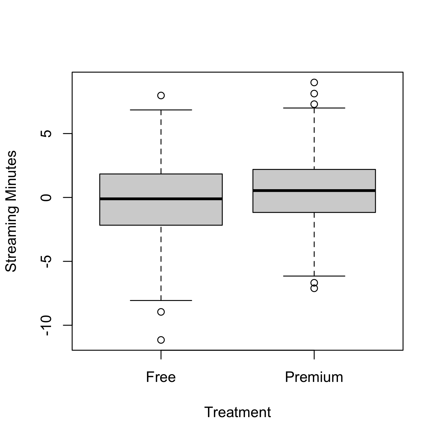
To see the effect of AccountType after adjusting for Age, we can plot the residuals from the regression of Age on Streaming Minutes.
From the above, we can see that the effect of account type on total streaming minutes, controlling for age, is now positive! However, even after controlling for age, can we be confident in interpreting this as a causal outcome of a hospital stay? The answer is still most likely no. That is because there may exist more confounding variables that are not a part of our data set; these are known as unobserved confounders. Even if there were no unobserved confounders, there are much more robust methods for analyzing observational studies than linear regression. We will discuss these in more detail in future posts.
Randomized Experiments
Randomized experiments remove the selection problem and ensure that there are no confounding variables (observed or unobserved). They do this by removing the individual’s opportunity to select whether or not they receive the treatment. In the Musicfi example, if we randomly upgraded some free accounts to premium accounts, then we would no longer have to adjust for age as (on average) there will be no age difference between the treated and control subjects.
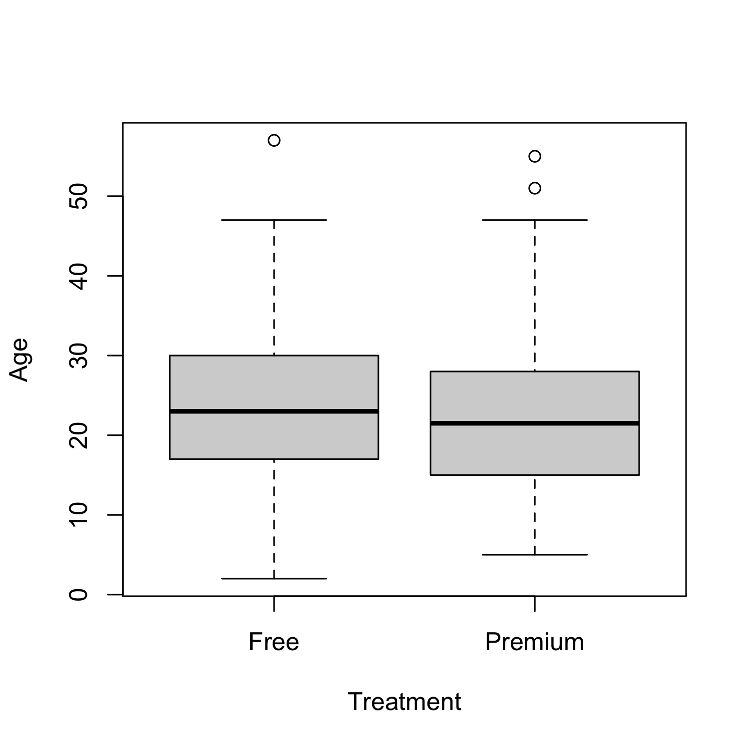
So even though age is still correlated with the amount of music that Musicfi customers listen to:
Age is not a confounding variables as it is indepedent of the treatment assignement. We can now directly attribute any differences in the outcome due to the intervention. Allowing us to conclude that giving people a premium account increases streaming minutes.
| |
In addition to ensuring that on average all covariates are balanced (i.e., the same) randomization also provides a basis for assumption light inference as we’ve discussed in our post on Randomization Based Inference: The Neymanian approach and Randomization-based inference: the Fisherian Approach.