Randomization-based inference: the Fisherian Approach

Why another approach to inference?

The limits of the Neymanian approach

The Neymanian approach to inference allows us to construct asymptotic confidence intervals for the average treatment effect under very mild assumptions. However, it has three main downsides (we will discuss these in more details in a subsequent post):

1. It can only be used with certain assignment mechanisms.
2. It is valid only asymptotically.
3. It still makes some assumptions (however mild they are).

How far can we get with no assumptions whatsoever?

Here, we briefly introduce an alternative approach to inference named after the famous Statistician R.A. Fisher. In contrast to the Neymanian approach to inference, the Fisherian approach:

1. Works with any assignment mechanism.
2. Is valid for any sample size \(n\).
3. Makes absolutely no assumptions whatever.

Now this looks an aweful lot like a free lunch, and we all know that the universe is never quite so cooperative — so what’s the catch?

Well, the downside is that in its simplest instantiation, this approach to inference does not give us an estimator of the average treatment effect, let alone a confidence interval. Instead, it allows us to answer the admittedly simpler question: based on the data, would it be reasonable to conclude that the treatment does not affect any of the units in the population. In statistical language, the Fisherian approach to inference allows us to test the following null hypothesis:

\[ H_0: \,Y_i(0) = Y_i(1) \quad \forall i=1,\ldots,n \]

At this point, it’s essential to understand what you need to assume with each inferential approach and what you get in exchange. The Fisher Randomization Test, as the Fisherian approach is often called, makes fewer assumptions than the Neymanian approach (in fact, it makes no assumptions whatsoever) — but the question it answers is, in a sense, narrower than that answered by the Neymanian approach.

Hypothesis testing as stochastic proof by contradiction

How can we test the null hypothesis \(H_0\) introduced above? If you’ve taken an introductory statistics class, you may have seen things like t-tests and chi-square tests, but it’s unclear how to apply these to test \(H_0\).

At this point, it is helpful to step back and consider what a statistical hypothesis testing is; a particular fruitful analogy is with a mathematical device called a proof by contradiction.

Suppose you wish to prove that a statement \(P\) is true. The idea of the proof by contradiction is to

1. Suppose that the opposite of \(P\) is in fact true.
2. Show that this leads to an internal contradiction, or an absurd statement.
3. Concludes that since the opposite of \(P\) leads to an absurdity, \(P\) must be true.

Example (from Wikipedia):

A famous example is the proof of the fact that there exists no smallest positive rational number. This is easy to show with a proof by contradiction. Indeed, suppose that there exists smallest positive rational number \(r = \frac{a}{b} > 0\). Then the number \(r’ = r/2 = \frac{a}{2b} > 0\) is also a positive rational number, but we have \(r’ < r\). This, however, contradicts the fact that \(r\) is the smallest positive rational number! We conclude that the initial supposition is wrong, and that there doesn’t exist a smallest positive rational number.

We can think of statistical hypothesis testing as a stochastic version of proof by contradiction. When we “test” the null hypothesis \(H_0\), our goal is to establish that it is false (or unlikely). Indeed, we can never verify the null hypothesis; we can only reject it or fail to reject it. By analogy with the proof by contradiction, the general strategy for hypothesis testing is as follows:

1. Suppose that \(H_0\) is true.
2. Show that this implies something very unlikely.
3. Conclude that since \(H_0\) leads to something very unlikely, it is unlikely to be true.

The key difference here is in step 2: showing that something is impossible is generally two stringent a criterion in statistics, so we settle for showing that it is unlikely.

The Fisher Randomization Test

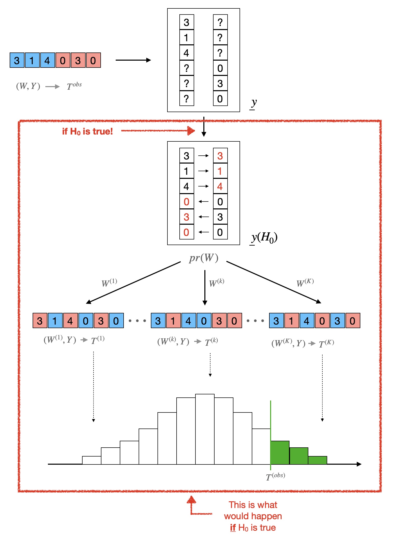
The Fisher randomization test begins with the observed assignment vector \(W\), the observed outcome vector \(Y\), and the sharp null hypothesis \(H_0\). Following the stochastic proof by contradiction analogy, let’s suppose for a moment \(H_0\) is, in fact, correct, and let’s follow the thread of implications.

Step 1: Hypothesized science table

If \(H_0\) is true, then we know the entire science table! Indeed, for illustration, suppose that \(W = (1, 1, 0, 1, 0, 0)\) and \(Y = (3, 1, 2, 1, 3, 0)\) as in our post on theNeymanian apprach. Again, we assume that the assignment was a completely randomized design with paramter \(n_1 = 3\).

As we’ve discussed in earlier posts, we typically only have a partial view of the science table since, as for each unit, we only observe one of the two potential outcomes. That is, we observe the following partial table:

But if \(H_0\) is true, then \(y_i(1) = y_i(0)\) for all units \(i\)! So each question mark in the table can be filled replaced by the number on the same row in the other column. That is, we have the following table:

Now we must be very careful. The science table above is not the true science table — it is the what the true science table would be if \(H_0\) where true! To make the distinction clear, we denote by \(\underline{y}(H_0)\) this hypothesized science table.

Step 2: Null distribution

Recall that our goal – in a stochastic proof by contradiction – is to show that supposing that \(H_0\) is true implies something very unlikely. One way to do so is to check whether “the outcome of the experiment we actually observe would be considered unusually extreme if \(H_0\) really were true.” Concretely, take any summary \(T\) of the observed data \(Y, W\) — we call this summary a “test statistic.” A simple choice, for instance, could be the average outcome of the treated units,

\[ T_a^{obs} = T_a(Y, W) = \frac{1}{n_1} \sum_{i=1}^n Y_i W_i, \]

or the difference in means,

\[ T_b^{obs} = T_b(Y, W) = \frac{1}{n_1} \sum_{i=1}^n Y_i W_i - \frac{1}{1-n_1} \sum_{i=1}^n Y_i (1-W_i). \]

In our specific example, we have \(T_a^{obs} = 5/3\) and \(T_b^{obs} = 5/3 - 5/3 = 0\). The choice of test statistic is important in practice — but it doesn’t affect the mechanics of the test so, for the sake of illustration, we will use \(T_b\) here. Now say we observe a certain value \(T_b^{obs}\) corresponding to the observed data \(Y, W\). Is this value surprising, if \(H_0\) is true? Well, we can check that. Suppose that we had observed assignment \(W^{(1)} = (1,1,1,0,0,0)\) instead. If \(H_0\) is true, then the science is \(\underline{y}(H_0)\), and so we would have observed \(Y^{(1)} = (3,1,2,1,3,0) \) and the corresponding value of the test statistic

\[ T_b^{(1)} = T_b(Y^{(1)}, W^{(1)}) = 4/2 - 6/2 = - 1 \]

Likewise for any possible assignment \(W^{(k)}\), we can deduce from \(\underline{y}(H_0)\) what \(Y^{(k)}\) and, therefore, \(T^{(k)}\) would have been. The distribution of \(T(y(W’), W’)\) under \(H_0\) is called the null distribution.

Step 3: p-values quantify our surprise

We now compare the value \(T^{obs}_{b}\) that we actually observe with the null distribution and ask: Is \(T^{obs}_b\) extreme compared to the other values or not? Specifically, we can ask how likely would it have been to observe a value as large as or larger than \(T^{obs}_b\) if \(H_0\) where true. This is what we call (one-sided) a p-value; formally

\[ pval(Y, W) = \sum_{W’} pr(W’) \cdot \mathbb{I}(T_b^{obs} \geq T(y(W’), W’)). \]

Step 4: interpreting the p-value

Now that we have obtained a p-value, let’s step back and see what it actually means, and how it fits into our general perspective of the Fisher Randomization Test as a stochastic proof by contradiction. To “disprove” \(H_0\), we assumed it to be true, and computed the probability of observing a value \(T_b\) more extreme than the one we actually observed; this was given by \(pval(Y, W)\). If \(pval(Y, W)\) is small—typically smaller than 0.05 or 0.01— we can reject the null hypothesis; otherwise, we fail to reject the null.

Summary of the Fisher Randomization Test

There is lot more that could be said about the Fisher Randomization Test — and indeed, we will say more about it in another post — but these are the very basics. The figure below summarizes the whole process

Convince yourself!

Once you really understand it, the Fisher Randomization Test is a profoundly beautiful — and useful — inferential tool. But even more so than the Neymanian approach to inference, it takes some getting used to. And here again, playing with simulations and implementing your own tests will really make a difference.

A simple implementation

The code below implements a simple – exact Fisher Randomization Test.

 1
 2
 3
 4
 5
 6
 7
 8
 9
10
11
12
13
14
15
16
17
18
19
20
21
22
23
24
25
26
27
28
29
30
31
32
33
34
35
36
37
38
39
40
41
42
43
44
45
46
47
48
49
50
51
52
53
54
55
56
57
58
59

library(magrittr)
library(purrr)
library(gtools)


## ----------------------------
## Test Statitsic
## ----------------------------

## Two examples of test statistics:
## Any function of w and y will do, so feel free to experiment!

T.1 <- function(w, y) mean(y[w==1]) - mean(y[w==0])
T.2 <- function(w, y) sum(y[w==1])


## ----------------------------
## Observed data
## ----------------------------

W.obs  <- c(1, 1, 0, 1, 0, 0)                  
Y.obs  <- c(3, 1, 2, 1, 3, 0)

T.1.obs <- T.1(W.obs, Y.obs)
T.2.obs <- T.2(W.obs, Y.obs)


## ----------------------------
## Constructing the null science
## ----------------------------

science.0 <- data.frame(y1 = Y.obs,
                        y0 = Y.obs)

## ----------------------------
## Computing the p-value -- the exact version
## ----------------------------

W.ls <- permutations(6, 6, 1:6) %>% 
    array_tree(1) %>% 
    map(~ W.obs[.]) %>% 
    unique

T.1.ls  <- vector('numeric', length=length(W.ls))
T.2.ls <- vector('numeric', length=length(W.ls))

for(i in seq_along(W.ls)) {
    W <- W.ls[[i]]
    Y <- science.0$y1 * W + science.0$y0 * (1-W)
    T.1.ls[i] <- T.1(W, Y)
    T.2.ls[i] <- T.2(W, Y)
}

pval.1 <- mean(T.1.ls >= T.1.obs)

pval.2 <- mean(T.2.ls >= T.2.obs)

One thing that may be surprising, when looking at the code, is that the true science table appears nowhere! That’s right, the pvalues we obtain at the end do depend on the true science only through the observed outcomes! Another insight — which see if you try the code with different values of Y.obs and W.obs is that pval.1 and pval.2 are always equal! That is a special property of the test statistics T.1 and T.2, but is not true in general.

You should play around with the code above, changing the values of W.obs and Y.obs (make sure that they remain vectors of lengths 6). Here are two useful exercises:

1. Come up with values of W.obs and Y.obs that yield high p-values.
2. Come up with values of W.obs and Y.obs that yield low p-values.

A fancier implementation

As mentioned earlier, one can think of the FRT as simply an algorithm that takes four inputs: the observed assignments, the observed outcomes, a test statistic, and the design of the experiment. We will show how to implement such an algorithm in the simple case where the design is completely randomized.

Before we do that, however, we point out another insight you can get from playing with the code above. You will notice that the value of Y in the loop on line 50 of the code is constant, and always equal to Y.obs. You can verify easily that this is true mathematically. This simple observation will allow us to simplify the code slightly. Below, an implementtion of the Fisher Randomization Test function:

 1
 2
 3
 4
 5
 6
 7
 8
 9
10
11
12
13
14
15
16
17
18
19

FRT <- function(Y.obs, W.obs, T) {
    ## Implementation of the FRT
    ## Y.obs: the vector of observed outcomes
    ## W.obs: the vector of observed assignments
    ## T: the test statistic. Must be a function T(., .)
    ##
    ## This function assumes that W was completely randomized,
    ## and returns a one sided p-value.

    W.ls <- permutations(length(W.obs), length(W.obs), 1:length(W.obs)) %>%
        array_tree(1) %>%
        map(~ W.obs[.]) %>%
        unique

    T.obs <-  T(W.obs, Y.obs)
    T.ls <- map_dbl(W.ls, ~T(., Y.obs))

    return(mean(T.ls >= T.obs))
}

This implementation uses map_dbl and the ~ from the purrr package to avoid having to wrap a loop, and uses the aforementioned fact that Y and Y.obs are always equal.

You will notice that although conceptually profound, the FRT can ultimately be implemented with just a few lines of code!

The FRT in practice: a Monte-Carlo approximation

Two practical problems with our implementation

If you’ve tried to modify the code above to run the FRT test in a setting with more that a dozen units, you will have noticed that the execution time rapidly becomes alarmingly long. The culprit is the line:

1
2
3
4

W.ls <- permutations(length(W.obs), length(W.obs), 1:length(W.obs)) %>%
        array_tree(1) %>%
        map(~ W.obs[.]) %>%
        unique

That generates all the assignments. Think about it for a moment: the support of a completely randomized design with \(n\) units, of which \(n_1\) are treated, has size \(n \choose n_1\).

• For \(n=10\) and \(n_1=5\), that’s 252 assignments: totally doable.
• For \(n=20\) and \(n_1 = 10\), that’s \(184,756\) assignments: still doable, but much slower.
• For \(n=30\) and \(n_1 = 15\), the support has more than \(10^8\) assignments: you should probably not try that on your laptop.

Another problem with our implementation is that it only allows us to run FRTs for completely randomized experiment — but the theory has no such requirements!

One solution

We can solve the first computational problem by approximate the null dsitribution by using only a subset of the possible assignments.

For the second problem, we can replace the permutations by any generic assignment mechanims. The sudo code is below.

 1
 2
 3
 4
 5
 6
 7
 8
 9
10
11
12
13
14
15
16
17
18

FRT.generic <- function(Y.obs, W.obs, T, Mechanism, iterations) {
    ## Implementation of the FRT
    ## Y.obs: the vector of observed outcomes
    ## W.obs: the vector of observed assignments
    ## T: the test statistic. Must be a function T(Y, W)
    ## Mechanism: a function that returns a new assignment W from the same
    ##            distribution as W.obs 
    ## iterations: the number of samples to obtain from the assignment
    ##             mechanism
    ##
    ## This function returns a one sided p-value.

    W.ls <- apply(Mechanism, iterations)
    T.obs <-  T(W.obs, Y.obs)
    T.ls <- map_dbl(W.ls, ~T(., Y.obs))

    return(mean(T.ls >= T.obs))
}