People don’t always agree; that is a fact of life. Similarly, when running an experiment, not everyone has the same reaction to the intervention! It’s critical that data scientists, academics, and the general public understand that the global average may not always be the most important or meaningful measure. Instead, it is often more informative to study how the effect of an intervention varies across different population subgroups. This post explains, at a high level, what heterogeneous treatment effects are, why they are essential, and how to think about them.
What are heterogeneous treatment effects?
Intuitive definition
When analyzing a randomized experiment or observational study, analysts often report the population average treatment effect (ATE) as the main —and often only— summary for the causal effect of the intervention. But what does it really mean? And who does it apply to? Just because we see that an intervention has a +1 (statistically significant) effect on average, can we conclude that the treatment would have an effect of +1 on every untreated unit, if we were to treat them? In short, the answer is no. The average is an important summary, but it often fails to provide the full picture. For example, an ATE of +1 may correspond to a scenario in which the intervention affects every unit equally; but it may also correspond to a case in which it has a +2 effect for half the units and -1 for the other half (see the figure below).
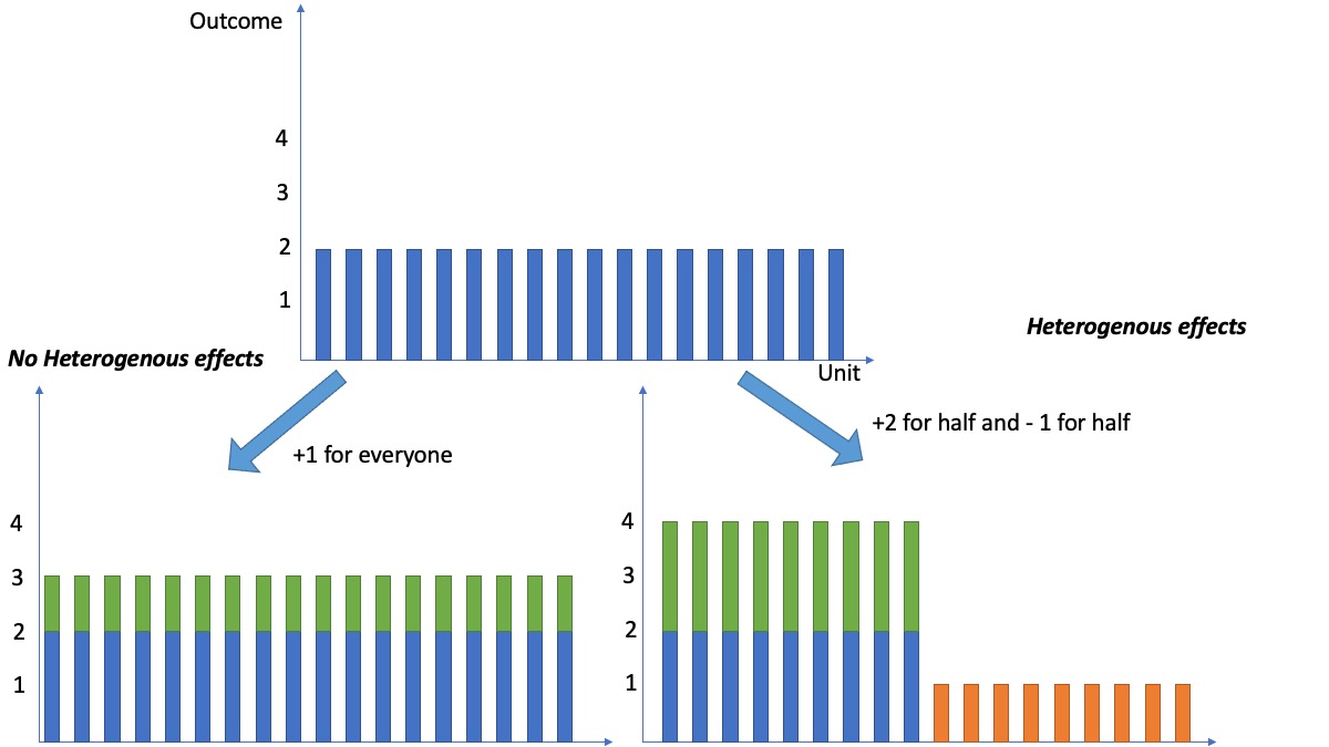
The figure illustrates how two different interventions can produce the same average causal effect. The left shows everyone having the same reaction to the intervention, whereas the right shows that some units have very positive responses and others have an adverse reaction.
Hetoregenous literally means “diverse in character or content,” so when we talk about “heterogeneous treatment effects,” we acknowledge the fact that every experimental unit may have a different response to the intervention. In practice, however, it is extremely difficult to reliably assess the effect of the intervention on each individual unit, and we must instead settle on assessing the effect of the intervention on subgroups of units that share similar characteristics. For example, it is common in clinical trials to report separate estimates for how a drug impacts children and for how it impacts adults, to reflect the biological differences. Technology companies similarly track responses across different platforms and countries.
Which heterogeneous effects to look at?
Any collection of average effects on subgroups of the population can be considered heterogeneous effects. Typically, the subgroups are defined by looking at each unit’s covariates (or characteristics). The extreme case is the individual treatment effects that try to ascertain each experimental unit’s causal effect separately; these, however, are virtually impossible to estimate without making strong assumptions. So what is the right middle ground between the average treatment effect (which is easy to estimate but not very informative) and the individual treatment effects (which are very informative but hard to estimate)? There is no unique answer to this question as it depends on the context. One crucial tradeoff to remember is that the smaller the subgroups we consider, the more difficult it is to estimate that subgroup’s effect.
Broadly speaking, there are two approaches to looking for heterogeneous treatment effects. The first requires knowledge of which groups to look at, and the second attempts to learn them from the data.
Estimating heterogeneous effects within pre-specified groups
Design Considerations
If we expect that some groups will react differently to our intervention, we can separate them before starting the experiment. In other words, we can run smaller-scale experiments within the pre-defined groups. That way, we can obtain separate estimates of the causal effects within the groups. For example, suppose you work at a technology company that has a presence in many countries. In that case, it is relatively common to separately run experiments within each country to ensure that we can estimate how the innovations are perceived differently across different geographies.
Post experiment analysis
We can estimate heterogeneous effects even when experiments where not run separately in each subgroup. Imagine we have a single binary covariate (for example, whether or not someone likes pie or whether or not someone is under the age of 18) that was recorded before the treatment assignment. Then, it is easy to measure the effect within the different values of this covariate. We simply group the units that like pie and the units that dislike pie and separately compute each group’s effect. We can carry out inference in the standard way, as discussed in our post on the potential outcomes framework. But, since we are testing multiple hypotheses, we need to perform a multiple comparison test adjustment to ensure that we control the overall type I error at the appropriate level. The simplest way to do this is via the Bonferroni correction that divides the nominal type I error by the number of tests.
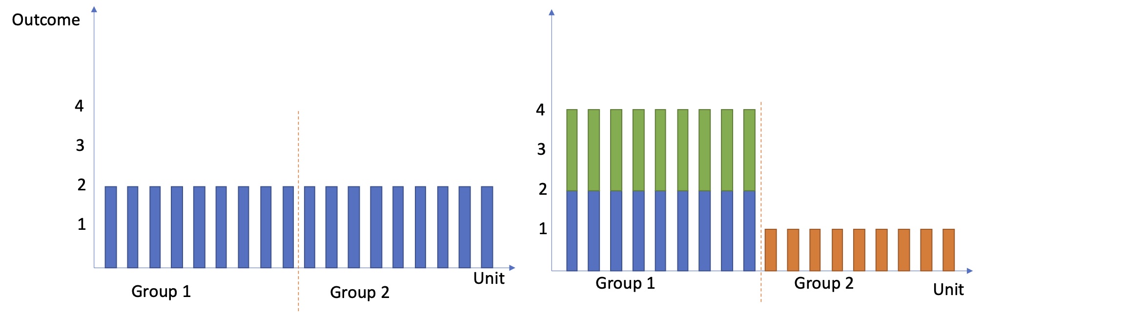
The figure shows the potential outcomes for two distinct groups of units. The left shows the control outcomes, and the right shows the treatment outcomes. Group 1 loved the intervention, whereas group 2 isn't as keen.
The post-experiment analysis approach works well with large experiments. However, depending on the adopted design, it might be the case that some groups are disproportionately assigned to certain treatments, making it hard to assess the heterogeneous effect accurately. That is why it is generally better to account for the subgroups of interest directly in the design, as suggested above.
Group discovery
The pre-specified strategy works well when there is only a handful of known groups. However, it starts to break down when the number of possible groups becomes large, which is often the case if we are interested in understanding how the effects differ across interactions of multiple covariates (i.e., children that like pie and adults that don’t like pie). When there are many possible groupings, and we don’t know which to look at, there is rarely enough data to perform an exhaustive search, so we have to be more strategic about finding these groups.
There are two intuitive approaches to accomplish. The first begins with the whole population and sequentially tries to split the sample into subgroups that reacted similarly to the intervention but differently from everyone else. The second starts with everyone in small groups and carefully combines the groups that reacted similarly to intervention until we have a manageable number of distinct groups such that, within the groups, the units responded similarly, but across groups, there are significant differences in the effect. See the two examples below for more details.
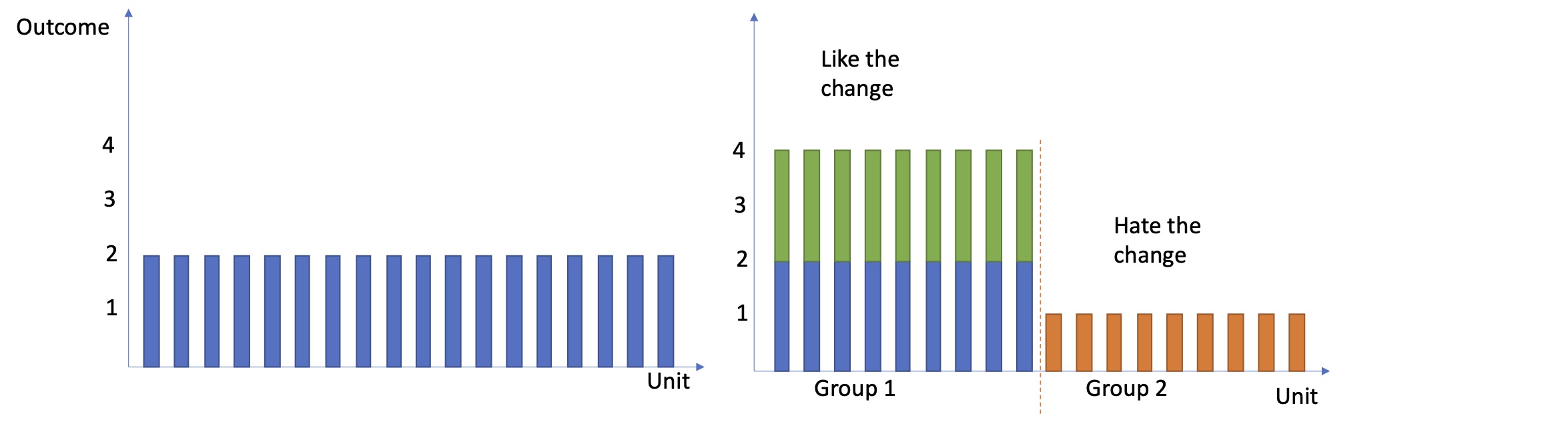
The figure shows the potential outcomes for a set of ungrouped units. The left shows the control outcomes, and the right shows the treatment outcomes. Based on the treatment effect, we can identify two distinct groups: Group 1 loved the intervention, and group 2 didn't.
Example 1: Split the data (Wager & Athey, 2018):
The machine learning community has widely used tree-based methods for both classification and regression tasks. Typically, these methods aim to partition covariate space into a set of homogeneous rectangles and then fit a simple model on each. The partitioning is done by finding a point that minimizes the within-group variability of the outcome. In causal inference, we focus on the causal effect; thus, applying this idea requires simply augmenting the objective function to find subgroups with estimated causal effects different from the overall group. This approach works well on small to moderate size data sets; however, the computation time increases rapidly as the data’s dimensions grow. This method is described in detail in Wager & Athey (2018) and is implemented in the grf R package (Athey et al. 2019).
Example 2: Regroup the data (Sepehri & DiCiccio, 2020):
An alternative to the above approach that tries to group the data by sequentially splitting the larger group into smaller groups is to reverse this. In particular, we can begin by grouping everyone into a fixed number of predefined subgroups based on their covariates. We then iteratively merge the two “most similar” clusters at each step until a stopping criterion is met. The notion of similarity and the stopping criteria can be defined using a formal hypothesis test; the resulting algorithm easily scalable to massive data sets and provide inferential guarantees about the output. This method is described in detail in Sepehri and DiCiccio (2020).
References
Athey, S., Tibshirani, J., & Wager, S. (2019). Generalized random forests. The Annals of Statistics, 47(2), 1148-1178.
Sepehri, A., & DiCiccio, C. (2020). Interpretable Assessment of Fairness During Model Evaluation. arXiv preprint arXiv:2010.13782.
Wager, S., & Athey, S. (2018). Estimation and inference of heterogeneous treatment effects using random forests. Journal of the American Statistical Association, 113(523), 1228-1242.